How InfoNCE Creates Exploration: The Hidden Engine of Contrastive RL
A personal exploration of the mechanisms behind emergent exploration in goal-conditioned reinforcement learning
Contrastive RL made a huge splash at NIPS 2025, with "1000 Layer Networks for Self-Supervised RL: Scaling Depth Can Enable New Goal-Reaching Capabilities". In this paper, the Princeton team demonstrated deep neural networks solving RL problems for the first time. Previous RL algorithms used very shallow networks, and so this discovery has the potential to unlock scaling laws for RL Agents.
A Fundamentally Different Paradigm
However, in my opinion most exciting thing about contrastive RL isn't its scalability—it's that it represents a fundamentally different paradigm for AI.
Traditional reinforcement learning creates a value function describing the value of a state in pursuit of a single objective. Contrastive RL creates something far more powerful: a coordinate transform which maps observations to a reachability metric for any state visited by the policy in the state space. This metric can then be used by the agent to pursue any goal.
Think about that. Instead of learning "how valuable is this state for reaching goal G?", the agent learns "how reachable is any state from any other state under my policy?" The representation itself becomes a universal navigation system, input the desired state, and voila!
Not only is it a more powerful paradigm, but initial results appear to show it learns faster than traditional RL. Why?
The answer emerged from a practical question: if we can learn to reach any goal, which goal should we collect data under? Should we use a curriculum of progressively harder goals? Sample random goals? The conventional wisdom suggested that goal selection would be critical—start easy, gradually increase difficulty.
But then came a surprising empirical finding: a single, fixed, hard goal works just as well. Sometimes better. This was documented in "One Goal is All You Need" (Liu, Tang, Eysenbach, 2024).
This is bizarre. A single hard goal means sparse reward—the agent wanders randomly until it accidentally reaches the goal, which might never happen. For traditional RL, sparse reward is death. Montezuma's Revenge is the canonical example: random trajectories never hit a reward, so there's no learning signal at all.
The field has developed three main approaches to this problem:
- Reward shaping - manually designing intermediate rewards (comes with its own issues)
- Behavior cloning - bootstrapping from demonstrations (AlphaGo used this, but AlphaZero later outperformed it without BC)
- Novelty-seeking algorithms - intrinsic motivation, curiosity-driven exploration
Yet contrastive RL sidesteps this entirely. It solves sparse-reward tasks without reward shaping, without demonstrations, without explicit novelty bonuses. How?
The answer: contrastive RL appears to come with a built-in novelty-seeking exploration algorithm. Based on my experience, it's this property, above all others, that's responsible for its remarkable results.
This has not gone unnoticed. Eysenbach's lab at Princeton has turned some of the brightest minds available to look deeply into the mathematics behind this emergent exploration. The resulting insights are remarkable.
The Papers
Two recent papers directly tackle the question of why contrastive RL explores so effectively:
"One Goal is All You Need" (Liu, Tang, Eysenbach, 2024, arXiv:2408.05804) made the surprising empirical observation that single-goal contrastive RL explores just as well as multi-goal variants—sometimes better. This raised the question: where does the exploration come from?
"Demystifying the Mechanisms Behind Emergent Exploration in Goal-conditioned RL" (Bastankhah et al., 2025, arXiv:2510.14129) provides the theoretical answer. This paper proves theorems about how representations evolve under contrastive training and why this naturally creates exploration pressure.
Together, these papers offer our best current understanding of the exploration phenomenon.
The Authors' Hypothesis
The core hypothesis is elegantly simple:
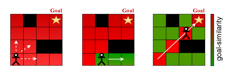
At initialization, all ψ representations are nearly the same—no temporal structure has been learned yet—so the goal-similarity c is high for all states. As training progresses, states along unsuccessful trajectories move away from ψ(g) in representation space.
In other words: everyone starts near the goal in representation space, and InfoNCE pushes visited states away. The actor, chasing goal-similarity, is forced toward the unexplored states that haven't been pushed away yet.
The paper frames this as a two-player game:
The Actor maximizes ψ(s)ᵀψ(g)—the inner product between the current state's representation and the goal's representation. Call this "ψ-similarity" or "goal-likeness."
The Critic optimizes InfoNCE loss, learning to discriminate reachable from unreachable state pairs. As a side effect, it pushes frequently-visited non-goal states away from the goal direction.
According to the theory, these two objectives create a self-sustaining exploration dynamic. The actor chases goal-similarity, while the critic keeps reducing goal-similarity for the states the actor visits. The agent is perpetually pushed toward novel regions.
The Key Tool: Vector Decomposition
The authors' key analytical tool is simple: decompose each state's representation in reachability space, relative to the goal direction.
Interactive visualization: Adjust the sliders to see how the raw c and ζ values get normalized onto the unit circle. Click "Animate" to see how growing ||ζ|| (from discrimination) squeezes c (goal similarity).
Any unit vector ψ(s) can be written as:
ψ(s) = c·z + ζ

where:
  z = ψ(g)         ← goal direction (unit vector)
  c = ψ(s)ᵀz       ← projection onto goal direction
  ζ = ψ(s) - c·z   ← orthogonal component
Under the SGCRL algorithms used in the paper, activations are normalized to unit vectors prior to being fed into the loss, so we have:
c² + ||ζ||² = 1
This constraint is everything. It's a zero-sum game between goal-alignment (c) and orthogonal structure (||ζ||). When one grows, the other must shrink.
The component c directly equals ψ-similarity: ψ(s)ᵀψ(g) = c. States with high c attract the actor. States with low or negative c are avoided.
The Mathematical Prediction
The theory's central prediction: during exploration, the goal direction gets squeezed and flattened.
Here's the mechanism:
During exploration, the goal is never in the training batch. InfoNCE trains on (state, future-state) pairs from trajectories. If we haven't reached the goal, ψ(g) never appears.
InfoNCE needs to discriminate positive from negative pairs. The goal direction z is shared—every state has some projection onto it. This shared component provides no discriminative signal. The orthogonal components ζ vary between states, so that's where the discriminative information lives.
Optimization follows the gradient signal. The ζ subspace has high variance, so InfoNCE optimization focuses there. Positive pairs align their ζ components; negative pairs spread theirs apart.
Normalization does the squeezing. As ||ζ||² grows from contrastive optimization, c² must shrink to maintain the unit norm constraint. Goal-similarity gets crowded out.
Theorem 2 formalizes this: under InfoNCE dynamics with symmetric initialization, c → 0 for states that appear in training batches. Visited states become orthogonal to the goal direction.
The result: frequently-observed states are pushed away from the goal, creating an exploration algorithm that strongly favors novel states.
The Tabular Experiment
Theory is one thing. Let's see what actually happens.
I recreated the papers tabular experiment of SGCRL (Single-Goal Contrastive RL) in a four-rooms maze. The agent starts in one corner, the goal is in the opposite corner, and every state has a learned 64-dimensional representation. The important thing here, there is no neural network in play. Each cell of the table is updated purely by the SGCRL loss.
Figure: Left panel — Gridworld where blue indicates states closer to the goal and red indicates states farther away. Right panel — Representation space where the c-axis shows cosine similarity to the goal (positive = closer), and ζ·PC₁ and ζ·PC₂ are the first and second principal components of the orthogonal residual in representation space.
What We Observe
The good news:
Frequently-visited states get pushed away from the goal. Watch the maze coloring evolve—states near the start turn red (low/negative c) while unexplored regions stay blue (high c). The agent is forced toward novelty.
Distance in the principal component grows faster than in the goal direction. The representations spread dramatically in the orthogonal subspace while the goal-direction variance compresses.
Clear clustering by reachability! The four rooms end up in distinct clusters, often completely opposite each other in the principal direction. The contrastive loss discovers the maze structure without any explicit topology information. This is remarkable.
The complications:
Random initialization fails. If we initialize representations randomly instead of symmetrically, the representation landscape becomes random, leading to random trajectories that suffer from the same sparse-reward problems as traditional RL. The symmetric initialization is load-bearing.
Unclear if the mechanism generalizes. The tabular experiment showcases the predicted behavior, but it's unclear if this is unique to the symmetric initialization or true in the general case. So let's try neural networks.
The Neural Network Implementation
I implemented an MLP version to see if the same dynamics emerge with function approximation.
A key thing I changed, was to represent the co-ordinates as two concatenated one-hot vectors, instead of just passing the integers to the network. This is because I found that the neural network perfectly represented the grid on initialization, due to the fact that the co-ordinates already encode the reachability. One hot vectors don't suffer from this problem, so we get a better test of the general case.
Different Behavior, Similar Outcomes
Here are my observations from spending a few hours watching runs:
With a one hot implementation and Xavier initialization, the states do indeed start close together, as the theory suggests.
Visited states are pulled apart from the unexplored states, and separated along the principal axis.
As training progresses, the goal direction receives random updates, which causes the entire representation to appear to "rotate" around the goal axis.
Since visited states are pushed to the edge, the rotation around the goal axis causes certain states to become highly attractive to the policy, resulting in cycles in the trajectory. The area around these cycles is explored. This leads to more accurate representations around the explored areas.
Continued random updates to the goal direction, cause rotation in the goal direction, which causes different attractors, which results in different exploration.
The discriminative loss pushes reachability clusters to different sides of the zeta (no goal) axis. For example, the top right room states all get mapped to +principal axis 1 and the bottom right get mapped to -principal axis 1. Eventually you clearly see the four rooms mapped to different parts of the space.
Random rotations around the goal axis, cause opposing reachability areas to become higher in the goal axis, resulting in exploration in all directions
This last point was the "aha" moment for me, where the theory and the practice came together. The normalization + the discriminative loss combined is what produces exploration, as the theory suggests. With no gradient in the goal direction, the normalization means that all points must be placed on a unit sphere, this results in the rotation effect. Since opposing reachable clusters should be on opposite sides of the axis, this rotation necessarily means that one's reachability groups loss must be another's gain, causing a different part of the space to be explored.
Finally, once the goal is sampled by the collection policy, the goal axis becomes fixed, and rotation in the goal axis ceases. Which halts exploration and heralds exploitation.
Conclusion: I'm a believer
At first, I had my doubts about this theory. However after going over the math and experiments for a few days, I think it's correct. The proof provided in the paper isolates the effect to the output normalization and loss function, and experiments support that this mechanism does transfer to the NN case. The main difference being that random rotation about the goal axis seems to be the driver of exploration in neural networks, as opposed to the pancake type flattening observed in the tabular case.
My thoughts
For single goals, we only need to set the goal to the collection policy and let the algorithm do the work. For multiple goals, it's less clear that this approach would work.. as setting a single goal will halt exploration in the collection policy once that goal is sampled.
In hard exploration environments, it's often difficult to tell if running the algorithm longer will have any effect. The theory provides us with some interesting ways to derive metrics that would tell us if exploration is proceeding. For example Hopkins statistics, nearest neighbour stats, or other metrics that characterise clusters in a high dimensional vector space. It may be worth providing the policy with subgoals and testing if it can reach them.
The 1000 Layer networks paper does not normalize the output to unit vectors. Instead, it uses a logsumexp loss penalty that penalizes the representation from having large values on a single axis. This will have a similar effect to normalizing to unit vectors, but the proof in the demystifying paper does not cover this case. So as always in good science, there are open questions that remain.
This is my first foray into the research, and the implications already seem revolutionary to me. Can't wait to dive in further!
References
Eysenbach, B., Zhang, T., Salakhutdinov, R., & Levine, S. (2022). Contrastive Learning as Goal-Conditioned Reinforcement Learning. NeurIPS 2022. arXiv:2206.07568
Liu, H., Tang, Y., & Eysenbach, B. (2024). One Goal is All You Need: Skills Can Emerge from Contrastive RL without Any Goal Sampling. arXiv:2408.05804
Bastankhah, M., et al. (2025). Demystifying the Mechanisms Behind Emergent Exploration in Goal-conditioned RL. arXiv:2510.14129
If you are interested in high-performance RL simulations, check out the Lightspeed project - a simulation framework built on the Madrona engine.
